Getting Started

Set up R and RStudio, and run your first lines of code

Installing the R Language and a Development Environment (IDE)

To follow along locally you need two free pieces of software:

R — the language itself. Download from cran.r-project.org.
RStudio — the editor (IDE). Download from posit.co/download/rstudio-desktop.

Install R first, then RStudio.

No installation needed on this site

Executable code blocks on this site run live in your browser via webR. Click Run Code to execute — no R or RStudio required.

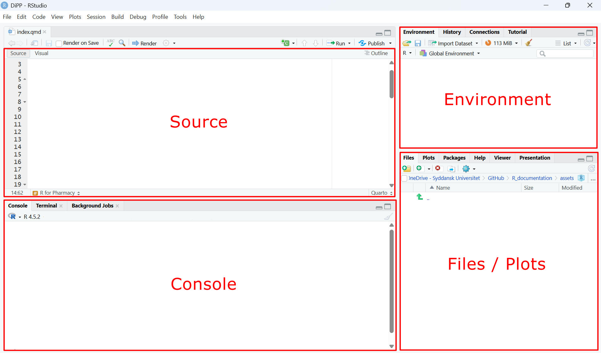
The RStudio interface

When you open RStudio you will see four panes:

Pane	Purpose
Source (top-left)	Write and save R scripts (files you write your code in)
Console (bottom-left)	Run code and see output
Environment (top-right)	See all objects currently in memory
Files / Plots (bottom-right)	Browse files, view plots, read help pages

Libraries / Packages

Packages are bundles of extra functions that extend what R can do. You download them once from CRAN (R’s central repository) and they’re stored locally in your library folder. The packages used throughout this site are mostly part of the tidyverse, a set of packages designed for data science.

Installing packages

Install packages once from CRAN using install.packages().

You install a package when you need functions it provides. Most functions you will need in the beginning are included in the tidyverse, so you can usually just install the tidyverse:

install.packages("tidyverse")

You only need to do this once per computer. So instead of writing it in your script and run the install every time you run your script, you can also execute the install in the console.

Loading packages

At the top of every script, load the packages you need with library(). This tells R which installed packages to make available in the current session.

library(tidyverse)

Note

Packages only need to be installed once, but must be loaded (library()) at the start of every new R session.

Data

Data is information that a computer can store and work with. It comes in different types — the most common ones you will encounter in R are:

Type	Example values	R type
Numbers	`74.2`, `3.14`	`numeric` / `double`
Whole numbers	`1`, `6`, `100`	`integer`
Text	`"PASS"`, `"batch_01"`	`character`
True/False	`TRUE`, `FALSE`	`logical`

Note

In R, decimal numbers use a . not a , — so three and a half is written 3.5, not 3,5.

The type matters because it determines what you can do with a value. You can calculate the average of numbers, but not of text.

In R, even a single value is stored as an object. When you have multiple values of the same type, they form a vector. And when you organize vectors into columns, you get a tibble — a modern version of a data frame with rows (observations) and columns (variables), similar to a table.

You create an object by assigning a value to a name using <-. On the left side of <-you write the name of your object (any name you choose). On the right side you write the data you want to store in that object.

temperature <- 22.5 
capital_city <- "Copenhagen"

Multiple values of the same type form a vector:

cities <- c("Copenhagen", "Aarhus", "Odense")
temperatures <- c(22.5, 19.3, 21.0)

And when you organize vectors into columns, you get a tibble. Since a tibble is a function from the tidyverse, remember to load the library:

library(tidyverse)

weather <- tibble(
  city        = cities,
  temperature = temperatures
)

Note

Object names must not contain spaces. Use _ instead, e.g. air_temperature. Choose meaningful object names that describe what is stored and, where relevant, include the unit. E.g., dose_mg instead of value.

Data is read into R from files using functions like read_csv().

Within RStudio, you can inspect your data objects in the Environment panel, or using

View(name_of_your_object)

Comments and Operations

Comments

Lines starting with # are comments — R ignores them when running code. Use comments to explain what your code does:

# This is a comment — R will not execute this line
dose_mg <- 500   # you can also add a comment after code

Operators

An operator is a symbol that performs an action on one or more values. They cover assignment (<-), arithmetic (+, -, etc.), comparison (==, >, etc.), and the pipe (%>%).

Assignment operator

Operator	Meaning	Example	Result
`<-`	Assign a value to a name	`x <- 42`	`x` now stores `42`

Arithmetic operators

Operator	Meaning	Example	Result
`+`	Addition	`3 + 2`	`5`
`-`	Subtraction	`10 - 4`	`6`
`*`	Multiplication	`5 * 3`	`15`
`/`	Division	`20 / 4`	`5`
`^`	Exponentiation	`2 ^ 3`	`8`
`%%`	Modulo (remainder)	`7 %% 3`	`1`

Comparison operators

Used to test conditions — return TRUE or FALSE:

Operator	Meaning	Example	Result
`==`	Equal to	`5 == 5`	`TRUE`
`!=`	Not equal to	`5 != 3`	`TRUE`
`>`	Greater than	`7 > 3`	`TRUE`
`<`	Less than	`2 < 1`	`FALSE`
`>=`	Greater or equal	`5 >= 5`	`TRUE`
`<=`	Less or equal	`3 <= 2`	`FALSE`

Pipe Operator

The pipe takes the output of one step and passes it as the input to the next — read it as “and then”. This allows you to chain multiple operations into a readable sequence without creating intermediate objects.

Operator	Meaning	Example	Result
`%>%`	Pass result to next function	`data %>% filter(age > 18)`	Filtered data frame containing entries where age is larger than 18

Computation

In R, data and computation are kept separate. You first store your data in objects, and then write expressions that compute with those objects. This is different from working in Excel, where data and formulas are mixed together in the same cells. In R, your data stays fixed in its object — computation produces a new object, leaving the original unchanged.

dose_mg   <- 500      # data
weight_kg <- 70       # data

dose_per_kg <- dose_mg / weight_kg   # computation — dose_mg and weight_kg unchanged

However, it is possible to overwrite the content of objects if you assign a different value to an existing object.

weight_kg <- 70    # data
weight_kg <- 80    # overwrites the previous value — weight_kg is now 80

You can add or transform columns in a tibble using mutate():

A common application case for computing is when you calculate new values and add them as new columns in an existing tibble using mutate(). Assume capsules is a tibble you loaded before containing the column fill_mass_mg. You now add two columns ibu_mg and pct_label which store newly computed values.

library(tidyverse)

# Add computed columns to an existing tibble
capsules <- capsules %>%
  mutate(
    ibu_mg    = fill_mass_mg * 0.43,        # active ingredient
    pct_label = ibu_mg / 75.0 * 100         # % of label claim
  )

R is vectorised — operations apply to entire columns at once, with no need for loops.

Output

R produces output in three main ways: printing to the console, viewing objects, and plotting.

Print to Console

Use cat() to print labelled results with units to the console:

Always round at the point of printing — store intermediate values at full precision:

# ✓ Correct
pct_label <- ibu_mg / label_claim_mg * 100       # full precision stored
cat("Label claim:", round(pct_label, 2), "%\n")  # round only when printing

Use signif() for concentrations and masses (significant figures), and round() for percentages and fixed decimal places.

View Objects

Inspect a data object in the RStudio Environment panel, or open it as a table:

View(your_data_object)

Plotting

Visualize data using ggplot2:

ggplot(your_data_object, aes(x = fill_mass_mg, y = pct_label)) +
  geom_point()

Plots appear in the Plots panel in RStudio.

Workflow

A typical R script follows this pattern:

Load packages — library()
Read data — read_csv()
Compute — mutate(), filter(), summarise(), mean(), sd()
Output — cat(), View(), ggplot()

# 1. Load packages
library(tidyverse)

# 2. Read data
capsules <- read_csv("data/capsule_weights.csv")

# 3. Compute
capsules <- capsules %>%
  mutate(
    fill_mass_mg = mass_filled_mg - mass_empty_mg,
    ibu_mg       = fill_mass_mg * ibu_per_mg_powder,
    pct_label    = ibu_mg / label_claim_mg * 100
  )

# 4. Output
cat("Mean % label claim:", round(mean(capsules$pct_label), 2), "%\n")
cat("SD:",                 round(sd(capsules$pct_label),   2), "%\n")

Browse the function reference to see all covered functions.