Visualization
Create plots with ggplot2 — scatter, line, bar, and box plots.
ggplot layer logic
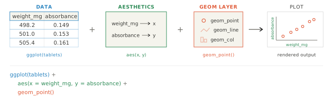
Every plot starts with ggplot(data, aes(...)) — this sets the data and axes. Add layers with +: geom_point(), geom_line(), labs(), theme_classic(). Order doesn’t matter for most layers, but theme_classic() always goes last.
- General chart gallery: The Data Visualization Catalogue
- R-focused chart chooser: From Data to Viz
- ggplot2 cheatsheet: Data visualization with ggplot2 - Cheat Sheet
Build a plot step by step
Step 1: Start with an empty plot object
This creates a blank ggplot canvas with no data or layers.
Step 2: Add data and map variables to axes with aes()
This connects the standards dataset and maps concentration to x and absorbance to y.
Step 3: Add points so the data is visible
This draws one point per observation using the x and y mappings.
Step 4: Add labels
This gives the plot a clear title and descriptive axis labels.
Step 5: Apply a theme to finalize the plot
This applies theme_classic() to set a clean visual style.
Scatter plot
Use geom_point() to plot individual observations as points.
Add a regression line with geom_smooth():
Line plot
Use geom_line() for data over time. Map colour to a grouping variable to show multiple batches.
Bar chart vs. Histogram
Bar chart
Use a bar chart geom_col() and geom_errorbar() to visualize summarized values (one value per category).
Histogram
Use a histogram geom_histogram() to visualize the distribution of many raw numeric observations.
- Bar chart: one bar per category, height is a known summary value.
- Histogram: bars represent bins of a continuous variable, showing frequency.
Box plot
Use geom_boxplot() to compare distributions across groups — ideal for batch comparisons.
- Center line in the box: the median (50th percentile).
- Bottom and top of the box: the 25th percentile (Q1) and 75th percentile (Q3).
- Box height: the interquartile range (IQR = Q3 - Q1), which contains the middle 50% of values.
- Whiskers: the most extreme values that are still within 1.5 x IQR from Q1 and Q3.
- Points beyond whiskers: outliers.
The example below includes a low outlier in Batch A and a high outlier in Batch B so you can see how outliers are shown.
Color, Shape, and transparency
Color and shape can separate groups, and transparency can reveal density when points overlap.
What is transparency (alpha)?
-
alphacontrols how see-through a geom is. -
Range:
alpha = 1means fully opaque;alpha = 0means fully transparent (invisible). - Lower alpha values help reveal where many points overlap, because darker regions indicate higher point density.
-
In practice, values around
0.2to0.5are often useful for dense scatter or jitter plots.
Tip: If you write geom_point(alpha = 0.3), all points get the same transparency. If you map alpha inside aes(...), transparency can vary by a variable.
Use color to encode groups
Map colour (points/lines) or fill (bars/boxes) to a variable when group identity matters. Try to use color with varying brightness (e.g. one darker and one lighter) or different hues (e.g. blue vs. orange) to make groups easy to distinguish. Varying brightness is often better for colorblind accessibility than varying hue.
Use color and shape to encode groups
To make your chart accessible for people with colorblindness, you can also map shape to a grouping variable.
Use transparency to reduce clutter
Lower alpha makes dense regions visible without hiding sparse points.
- Use color only when it communicates information, not decoration.
- Keep palettes simple and high-contrast.
- Use transparency when many points overlap.
Overplotting and how to fight it
Overplotting happens when many points overlap so heavily that patterns become hard to see.
You can fight this in many ways:
1) Use transparency (alpha)
Lower opacity reveals where points pile up.
2) Add jitter
Jitter spreads overlapping points so you can see repeated values.
3) Use visual abstraction
Sometimes the best fix is to summarize the data (for example with violin or box plots). See the next collapsible section, Visual abstraction: low to high.
Visual abstraction
Visual abstraction means how much of the raw data you keep visible. Lower abstraction shows individual observations; higher abstraction summarizes them.
Low abstraction: points (raw observations)
You can see every data point, which makes outliers and clusters easy to spot.
Medium abstraction: violin plot (distribution shape)
You lose exact points but gain a quick view of distribution shape and spread.
High abstraction: box plot (summary statistics)
You mainly see median, quartiles, and whiskers; individual points are hidden.
- Faster comparison across groups.
- Less visual clutter in large datasets.
- Highlights central patterns and spread.
- Can hide outliers or multimodal patterns.
- Can hide sample size differences.
- Too much abstraction can hide important details.